THE DATA LINK LAYER

Unit3: TheData-link layer 

Data-link layer is the second layer after the physical layer. The data link layer is responsible for maintaining the data link between two hosts or nodes. 

Design Issues in Data Link Layer

1. Services provided to the network layer – 
The data link layer act as a service interface to the network layer. The principle service is transferring data from network layer on sending machine to the network layer on destination machine. This transfer also takes place via DLL (Data link-layer). 

2. Frame synchronization :
The source machine sends data in the form of blocks called frames to the destination machine. The starting and ending of each frame should be identified so that the frame can be recognized by the destination machine.  

3. Flow control :
Flow control is done to prevent the flow of data frame at the receiver end. The source machine must not send data frames at a rate faster than the capacity of destination machine to accept them. 

4. Error control :
Error control is done to prevent duplication of frames. The errors introduced during transmission from source to destination machines must be detected and corrected at the destination machine. 

Error Detection in Computer Networks

Error
A condition when the receiver’s information does not match with the sender’s information. During transmission, digital signals suffer from noise that can introduce errors in the binary bits travelling from sender to receiver. That means a 0 bit may change to 1 or a 1 bit may change to 0. Error Detecting Codes (Implemented either at Data link layer or Transport Layer of OSI Model)
Whenever a message is transmitted, it may get scrambled by noise or data may get corrupted. To avoid this, we use error-detecting codes which are additional data added to a given digital message to help us detect if any error has occurred during transmission of the message.
Basic approach used for error detection is the use of redundancy bits, where additional bits are added to facilitate detection of errors.

Some popular techniques for error detection are:
1. Simple Parity check
2. Two-dimensional Parity check
3. Checksum
4. Cyclic redundancy check

1. Simple Parity check
Blocks of data from the source are subjected to a check bit or parity bit generator form, where a parity of :

1 is added to the block if it contains odd number of 1’s, and

0 is added if it contains even number of 1’s

This scheme makes the total number of 1’s even, that is why it is called even parity checking.

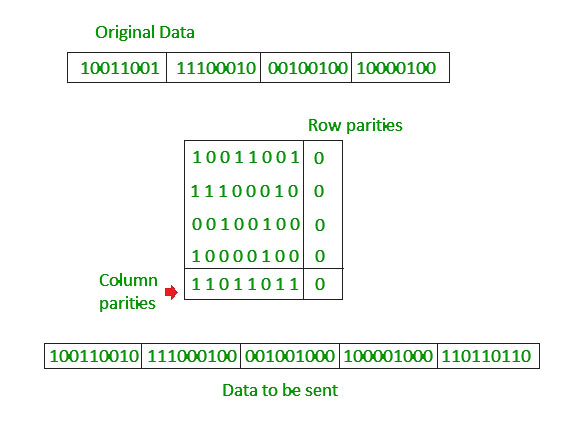
2. Two-dimensional Parity check

Parity check bits are calculated for each row, which is equivalent to a simple parity check bit. Parity check bits are also calculated for all columns, then both are sent along with the data. At the receiving end these are compared with the parity bits calculated on the received data.

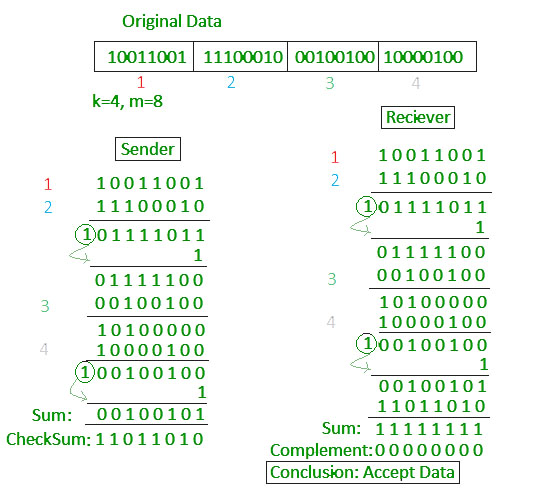
3. Checksum

·   In checksum error detection scheme, the data is divided into k segments each of m bits.

·   In the sender’s end the segments are added using 1’s complement arithmetic to get the sum. The sum is complemented to get the checksum.

·   The checksum segment is sent along with the data segments.

·   At the receiver’s end, all received segments are added using 1’s complement arithmetic to get the sum. The sum is complemented.

·   If the result is zero, the received data is accepted; otherwise discarded.

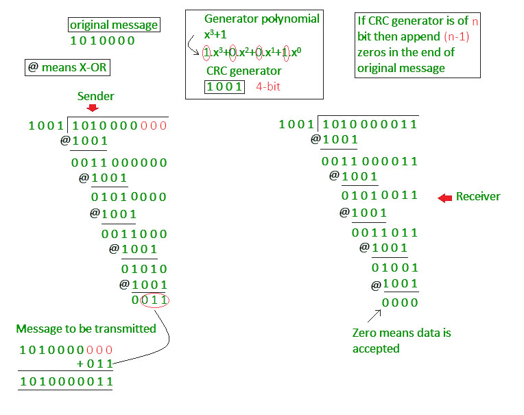
4. Cyclic redundancy check (CRC)

Unlike checksum scheme, which is based on addition, CRC is based on binary division.

In CRC, a sequence of redundant bits, called cyclic redundancy check bits, are appended to the end of data unit so that the resulting data unit becomes exactly divisible by a second, predetermined binary number.

·   At the destination, the incoming data unit is divided by the same number.

·   If at this step there is no remainder, the data unit is assumed to be correct and is therefore accepted.

 

·   A remainder indicates that the data unit has been damaged in transit and therefore must be rejected. 
Example :

 polynomial Code

A polynomial code is a linear code having a set of valid code words that comprises of polynomials divisible by a shorter fixed polynomial is known as generator polynomial.

They are used for error detection and correction during the transmission of data as well as storage of data.

Hamming Code in Computer Network

Hamming code is a set of error-correction codes that can be used to detect and correct the errors that can occur when the data is moved or stored from the sender to the receiver.

It is a technique developed by R.W. Hamming for error correction. 

·   Redundant bits – Redundant bits are extra binary bits that are generated and added to the information-carrying bits of data transfer to ensure that no bits were lost during the data transfer.

·   The number of redundant bits can be calculated using the following formula:

 2^r ≥ m + r + 1

 where, r = redundant bit, m = data bit

Suppose the number of data bits is 7, then the number of redundant bits can be calculated using: = 2^4 ≥ 7 + 4 + 1 Thus, the number of redundant bits= 4 Parity bits.  A parity bit is a bit appended to a data of binary bits to ensure that the total number of 1’s in the data is even or odd. Parity bits are used for error detection.

There are two types of parity bits:

Even parity bit: 

In the case of even parity, for a given set of bits, the number of 1’s are counted. If that count is odd, the parity bit value is set to 1, making the total count of occurrences of 1’s an even number. If the total number of 1’s in a given set of bits is already even, the parity bit’s value is 0.

Odd Parity bit :

In the case of odd parity, for a given set of bits, the number of 1’s are counted. If that count is even, the parity bit value is set to 1, making the total count of occurrences of 1’s an odd number. If the total number of 1’s in a given set of bits is already odd, the parity bit’s value is 0.

General Algorithm of Hamming code: 

Hamming Code is simply the use of extra parity bits to allow the identification of an error.

Write the bit positions starting from 1 in binary form (1, 10, 11, 100, etc).

All the bit positions that are a power of 2 are marked as parity bits (1, 2, 4, 8, etc).

All the other bit positions are marked as data bits.

Each data bit is included in a unique set of parity bits, as determined its bit position in binary form. a. Parity bit 1 covers all the bits positions whose binary representation includes a 1 in the least significant position (1, 3, 5, 7, 9, 11, etc). b. Parity bit 2 covers all the bits positions whose binary representation includes a 1 in the second position from the least significant bit (2, 3, 6, 7, 10, 11, etc). c. Parity bit 4 covers all the bits positions whose binary representation includes a 1 in the third position from the least significant bit (4–7, 12–15, 20–23, etc). d. Parity bit 8 covers all the bits positions whose binary representation includes a 1 in the fourth position from the least significant bit bits (8–15, 24–31, 40–47, etc). e. In general, each parity bit covers all bits where the bitwise AND of the parity position and the bit position is non-zero.

Since we check for even parity set a parity bit to 1 if the total number of ones in the positions it checks is odd.

Set a parity bit to 0 if the total number of ones in the positions it checks is even.

Determining the position of redundant bits – These redundancy bits are placed at positions that correspond to the power of 2. 

As in the above example:

The number of data bits = 7

The number of redundant bits = 4

The total number of bits = 11

The redundant bits are placed at positions corresponding to power of 2- 1, 2, 4, and 8

Suppose the data to be transmitted is 1011001, the bits will be placed as follows: 

Determining the Parity bits:

R1 bit is calculated using parity check at all the bits positions whose binary representation includes a 1 in the least significant position. R1: bits 1, 3, 5, 7, 9, 11 

To find the redundant bit R1, we check for even parity. Since the total number of 1’s in all the bit positions corresponding to R1 is an even number the value of R1 (parity bit’s value) = 0

R2 bit is calculated using parity check at all the bits positions whose binary representation includes a 1 in the second position from the least significant bit. R2: bits 2,3,6,7,10,11 

To find the redundant bit R2, we check for even parity. Since the total number of 1’s in all the bit positions corresponding to R2 is odd the value of R2(parity bit’s value)=1

R4 bit is calculated using parity check at all the bits positions whose binary representation includes a 1 in the third position from the least significant bit. R4: bits 4, 5, 6, 7 

To find the redundant bit R4, we check for even parity. Since the total number of 1’s in all the bit positions corresponding to R4 is odd the value of R4(parity bit’s value) = 1

R8 bit is calculated using parity check at all the bits positions whose binary representation includes a 1 in the fourth position from the least significant bit. R8: bit

8,9,10,11

To find the redundant bit R8, we check for even parity. Since the total number of 1’s in all the bit positions corresponding to R8 is an even number the value of R8(parity bit’s value)=0. Thus, the data transferred is:

Error detection and correction: Suppose in the above example the 6th bit is changed from 0 to 1 during data transmission, then it gives new parity values in the binary number: 

The bits give the binary number 0110 whose decimal representation is 6. Thus, bit 6 contains an error. To correct the error the 6th bit is changed from 1 to 0.

What are elementary data link layer protocols

Elementary Data Link protocols are classified into three categories, as given below −

Protocol 1 − Unrestricted simplex protocol

Protocol 2 − Simplex stop and wait protocol

Protocol 3 − Simplex protocol for noisy channels.

Unrestricted Simplex Protocol

Data transmitting is carried out in one direction only. The transmission (Tx) and receiving (Rx) are always ready and the processing time can be ignored. In this protocol, infinite buffer space is available, and no errors are occurring that is no damage frames and no lost frames.

The Unrestricted Simplex Protocol is diagrammatically represented as follows –

 

Simplex Stop and Wait protocol

In this protocol we assume that data is transmitted in one direction only. No error occurs; the receiver can only process the received information at finite rate. These assumptions imply that the transmitter cannot send frames at rate faster than the receiver can process them.

The main problem here is how to prevent the sender from flooding the receiver.

The general solution for this problem is to have the receiver send some sort of feedback to sender, the process is as follows

Step1 − The receiver send the acknowledgement frame back to the sender telling the sender that the last received frame has been processed and passed to the host.

Step 2 − Permission to send the next frame is granted.

Step 3 − The sender after sending the sent frame has to wait for an acknowledge frame from the receiver before sending another frame.

This protocol is called Simplex Stop and wait protocol, the sender sends one frame and waits for feedback from the receiver. When the ACK arrives, the sender sends the next frame.

The Simplex Stop and Wait Protocol is diagrammatically represented as follows

Simplex Protocol for Noisy Channel

Data transfer is only in one direction, consider separate sender and receiver, finite processing capacity and speed at the receiver, since it is a noisy channel, errors in data frames or acknowledgement frames are expected. Every frame has a unique sequence number.

After a frame has been transmitted, the timer is started for a finite time. Before the timer expires, if the acknowledgement is not received , the frame gets retransmitted, when the acknowledgement gets corrupted or sent data frames gets damaged, how long the sender should wait to transmit the next frame is infinite.

The Simplex Protocol for Noisy Channel is diagrammatically represented as follows

Sliding Window Protocol | Set 1 (Sender Side)

Prerequisite : Stop and Wait ARQ

The Stop and Wait ARQ offers error and flow control, but may cause big performance issues as sender always waits for acknowledgement even if it has next packet ready to send. Consider a situation where you have a high bandwidth connection and propagation delay is also high (you are connected to some server in some other country through a high-speed connection), you can’t use this full speed due to limitations of stop and wait.

Sliding Window protocol handles this efficiency issue by sending more than one packet at a time with a larger sequence number.

The idea is same as pipelining in architecture.

Few Terminologies :

Transmission Delay (Tt) – Time to transmit the packet from host to the outgoing link. If B is the Bandwidth of the link and D is the Data Size to transmit

    Tt = D/B 

Propagation Delay (Tp) – It is the time taken by the first bit transferred by the host onto the outgoing link to reach the destination. It depends on the distance d and the wave propagation speed s (depends on the characteristics of the medium).

   Tp = d/s 

Efficiency – It is defined as the ratio of total useful time to the total cycle time of a packet. For stop and wait protocol,

Total cycle time = Tt(data) + Tp(data) +

                    Tt(acknowledgement) + Tp(acknowledgement)

              =  Tt(data) + Tp(data) + Tp(acknowledgement)

         =   Tt + 2*Tp

Since acknowledgements are very less in size, their transmission delay can be neglected.

Efficiency = Useful Time / Total Cycle Time

           = Tt/(Tt + 2*Tp) (For Stop and Wait)

           = 1/(1+2a)  [ Using a = Tp/Tt ]

Effective Bandwidth(EB) or Throughput – Number of bits sent per second.

EB = Data Size(D) / Total Cycle time(Tt + 2*Tp)

Multiplying and dividing by Bandwidth (B),

       =  (1/(1+2a)) * B   [ Using a = Tp/Tt ]

       =  Efficiency * Bandwidth

Capacity of link – If a channel is Full Duplex, then bits can be transferred in both the directions and without any collisions. Number of bits a channel/Link can hold at maximum is its capacity.

 Capacity = Bandwidth(B) * Propagation(Tp)

For Full Duplex channels,

Capacity = 2*Bandwidth(B) * Propagation(Tp)

Concept of Pipelining

In Stop and Wait protocol, only 1 packet is transmitted onto the link and then sender waits for acknowledgement from the receiver. The problem in this setup is that efficiency is very less as we are not filling the channel with more packets after 1st packet has been put onto the link. Within the total cycle time of Tt + 2*Tp units, we will now calculate the maximum number of packets that sender can transmit on the link before getting an acknowledgement.

 In Tt units ----> 1 packet is Transmitted.

 In 1 units  ----> 1/Tt packet can be Transmitted.

 In  Tt + 2*Tp units ----->  (Tt + 2*Tp)/Tt

                             packets can be Transmitted

                ------>  1 + 2a  [Using a = Tp/Tt]

Maximum packets That can be Transmitted in total cycle time = 1+2*a

Let me explain now with the help of an example.

Consider Tt = 1ms, Tp = 1.5ms.

In the picture given below, after sender has transmitted packet 0, it will immediately transmit packets 1, 2, 3. Acknowledgement for 0 will arrive after 2*1.5 = 3ms. In Stop and Wait, in time 1 + 2*1.5 = 4ms, we were transferring one packet only. Here we keep a window of packets that we have transmitted but not yet acknowledged.

After we have received the Ack for packet 0, window slides and the next packet can be assigned sequence number 0. We reuse the sequence numbers which we have acknowledged so that header size can be kept minimum as shown in the diagram given below.

Minimum Number Of Bits For Sender window (Very Important For GATE)

As we have seen above,

Maximum window size = 1 + 2*a    where a = Tp/Tt

Minimum sequence numbers required = 1 + 2*a.

All the packets in the current window will be given a sequence number. Number of bits required to represent the sender window = ceil(log2(1+2*a)).

But sometimes number of bits in the protocol headers is pre-defined. Size of sequence number field in header will also determine the maximum number of packets that we can send in total cycle time. If N is the size of sequence number field in the header in bits, then we can have 2N sequence numbers.

Window Size ws = min(1+2*a, 2N)

If you want to calculate minimum bits required to represent sequence numbers/sender window, it will be ceil(log2(ws)).

In this article, we have discussed sending window only. For receiving window, there are 2 protocols namely Go Back N and Selective Repeat which are used to implement pipelining practically.

Sliding Window Protocol | Set 2 (Receiver Side)

Please refer this as a prerequisite article: Sliding Window Protocol (sender side)| set 1

Sliding Window Protocol is actually a theoretical concept in which we have only talked about what should be the sender window size (1+2a) in order to increase the efficiency of stop and wait arq. the practical implementations in which we take care of what should be the size of receiver window. Practically it is implemented in two protocols namely :

Go Back N (GBN)

Selective Repeat (SR)

Go Back N (GBN) Protocol

The three main characteristic features of GBN are:

Sender Window Size (WS)
It is N itself. If we say the protocol is GB10, then Ws = 10. N should be always greater than 1 in order to implement pipelining. For N = 1, it reduces to Stop and Wait protocol.

Efficiency Of GBN = N/(1+2a)

where a = Tp/Tt

If B is the bandwidth of the channel, then

Effective Bandwidth or Throughput

 = Efficiency * Bandwidth

 = (N/(1+2a)) * B

Receiver Window Size (WR)

WR is always 1 in GBN.

Now what exactly happens in GBN, will explain with a help of example. Consider the diagram given below. We have sender window size of 4. Assume that we have lots of sequence numbers just for the sake of explanation. Now the sender has sent the packets 0, 1, 2 and 3. After acknowledging the packets 0 and 1, receiver is now expecting packet 2 and sender window has also slided to further transmit the packets 4 and 5. Now suppose the packet 2 is lost in the network, Receiver will discard all the packets which sender has transmitted after packet 2 as it is expecting sequence number of 2. On the sender side for every packet send there is a time out timer which will expire for packet number 2. Now from the last transmitted packet 5 sender will go back to the packet number 2 in the current window and transmit all the packets till packet number 5. That’s why it is called Go Back N. Go back means sender has to go back N places from the last transmitted packet in the unacknowledged window and not from the point where the packet is lost.

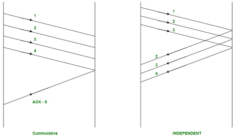
Acknowledgements
There are 2 kinds of acknowledgements namely:

Cumulative Ack: One acknowledgement is used for many packets. The main advantage is traffic is less. A disadvantage is less reliability as if one ack is the loss that would mean that all the packets sent are lost.

Independent Ack: If every packet is going to get acknowledgement independently. Reliability is high here but a disadvantage is that traffic is also high since for every packet we are receiving independent ack.

GBN uses Cumulative Acknowledgement. At the receiver side, it starts a acknowledgement timer whenever receiver receives any packet which is fixed and when it expires, it is going to send a cumulative Ack for the number of packets received in that interval of timer. If receiver has received N packets, then the Acknowledgement number will be N+1. Important point is Acknowledgement timer will not start after the expiry of first timer but after receiver has received a packet.
Time out timer at the sender side should be greater than Acknowledgement timer.

Relationship Between Window Sizes and Sequence Numbers
We already know that sequence numbers required should always be equal to the size of window in any sliding window protocol.

Minimum sequence numbers required in GBN = N + 1

Bits Required in GBN = ceil(log2 (N + 1))

The extra 1 is required in order to

avoid the problem of duplicate packets

as described below.

Example: Consider an example of GB4.

Sender window size is 4 therefore we require a minimum of 4 sequence numbers to label each packet in the window.

Now suppose receiver has received all the packets(0, 1, 2 and 3 sent by sender) and hence is now waiting for packet number 0 again (We cannot use 4 here as we have only 4 sequence numbers available since N = 4).

Now suppose the cumulative ack for the above 4 packets is lost in the network.

On sender side, there will be timeout for packet 0 and hence all the 4 packets will be transmitted again.

Problem now is receiver is waiting for new set of packets which should have started from 0 but now it will receive the duplicate copies of the previously accepted packets.

In order to avoid this, we need one extra sequence number.

Now the receiver could easily reject all the duplicate packets which were starting from 0 because now it will be waiting for packet number 4 (We have added an extra sequence number now).

This is explained with the help of the illustrations below.

Trying with Sequence numbers 4.

Now Trying with one extra Sequence Number.

Now it is clear as to why we need an extra 1 bit in the GBN protocol.

In the next article, we will explain Selective repeat and comparison between the 2 protocols.

Bottom of Form

Sliding Window Protocol | Set 3 (Selective Repeat)

Prerequisite : Sliding Window Protocol – Set 1 (Sender Side), Set 2 (Receiver Side) Why Selective Repeat Protocol? The go-back-n protocol works well if errors are less, but if the line is poor it wastes a lot of bandwidth on retransmitted frames. An alternative strategy, the selective repeat protocol, is to allow the receiver to accept and buffer the frames following a damaged or lost one. Selective Repeat attempts to retransmit only those packets that are actually lost (due to errors) :

Receiver must be able to accept packets out of order.

Since receiver must release packets to higher layer in order, the receiver must be able to buffer some packets.

Retransmission requests :

Implicit – The receiver acknowledges every good packet, packets that are not ACKed before a time-out are assumed lost or in error. Notice that this approach must be used to be sure that every packet is eventually received.

Explicit – An explicit NAK (selective reject) can request retransmission of just one packet. This approach can expedite the retransmission but is not strictly needed.

One or both approaches are used in practice.

Selective Repeat Protocol (SRP) : 

This protocol(SRP) is mostly identical to GBN protocol, except that buffers are used and the receiver, and the sender, each maintains a window of size. SRP works better when the link is very unreliable. Because in this case, retransmission tends to happen more frequently, selectively retransmitting frames is more efficient than retransmitting all of them. SRP also requires full-duplex link. backward acknowledgements are also in progress.

Sender’s Windows ( Ws) = Receiver’s Windows ( Wr).

Window size should be less than or equal to half the sequence number in SR protocol. This is to avoid packets being recognized incorrectly. If the size of the window is greater than half the sequence number space, then if an ACK is lost, the sender may send new packets that the receiver believes are retransmissions.

Sender can transmit new packets as long as their number is with W of all unACKed packets.

Sender retransmit un-ACKed packets after a timeout – Or upon a NAK if NAK is employed.

Receiver ACKs all correct packets.

Receiver stores correct packets until they can be delivered in order to the higher layer.

In Selective Repeat ARQ, the size of the sender and receiver window must be at most one-half of 2^m.

Figure – the sender only retransmits frames, for which a NAK is received Efficiency of Selective Repeat Protocol (SRP) is same as GO-Back-N’s efficiency :

Efficiency = N/(1+2a)

Where a = Propagation delay / Transmission delay 

Buffers = N + N

Sequence number  = N(sender side)  + N  ( Receiver Side)